强化学习基础

本文引用了莫烦大大和几位知乎答主的部分文字，由于时间较长，无法一一确认，在这里统一感谢。如有侵害到您版权的行为，请您尽快联系我修改，感谢。

Reinforcement Learning Basic

定义

强化学习涉及一个智能体，一组“状态”S和每个状态下的动作集合A。通过执行一个行动 ，该智能体从一个状态转移到另一个状态。在一个特定的状态下执行一个动作时，智能体还可以得到一个奖励。
智能体的目标是最大化其奖励的累加。这个潜在的奖励是所有未来可以拿到的奖励值的期望的加权和。

例如，假设现在你要上地铁，奖励就是你所花的时间的相反数。一种策略就是车门一开就往上挤，但是还有很多人要下车，逆着人流往上挤也会花费不少时间，这个时候你花的总时间可能是：

• 0秒钟等待时间+15秒挤上去的时间
  在接下来的一天，很巧合，你决定先让别人下车。虽然这个时候看起来等待的时间稍微增加了，但是下车的人也会下的更顺畅，这个时候你可能花的时间是：
• 5秒等待时间+0秒挤上去的时间。

理解

状态State和动作Action存在映射关系，也就是一个state可以对应一个action，或者对应不同动作的概率（常常用概率来表示，概率最高的就是最值得执行的动作）。状态与动作的关系其实就是输入与输出的关系，而状态State到动作Action的过程就称之为一个**策略Policy，**一般用π表示，也就是需要找到以下关系(其中a是action，s是state)：

一一对应表示：a=π(s)

概率表示：π(a|s)

基本方法对比

Method name	Net Classes Num	Net Num	Net types	Input	Output	Update method	Use Memory	Policy
Q-L	0	0		state	values of actions	round update	F	OFF
SARSA	0	0		state	value of actions	round update	F	ON
DQN	1	2	target net & Eval net	state	values of actions	round update	T
PG	1	1	policy net	state	prob of actions	round update	T
AC	2	2	actor net & critic net	state	prob of actions & rewards	step update	F	OFF
DDPG	2	4	(actor & critic)x(target & eval)	state & (state, action)	continuous action value & reward	step update	T	OFF

规律与注解

• 只定义了一个网络类的方法都是回合制更新
• 除了DDPG其他方法的输入都是state
• 回合制更新也叫蒙特卡洛更新（Monte-carlo update），单步更新也叫当时差距更新（Temporal-difference update）

Q-Learning

定义

Q-学习是强化学习的一种方法。Q-学习就是要学习的政策，告诉智能体什么情况下采取什么行动。Q-learning不需要对环境进行建模，即使是对带有随机因素的转移函数或者奖励函数也不需要进行特别的改动就可以进行。
对于任何有限的马可夫决策过程（FMDP），Q-learning可以找到一个可以最大化所有步骤的奖励期望的策略。[1]，在给定一个部分随机的策略和无限的探索时间，Q-learning可以给出一个最佳的动作选择策略。“Q”这个字母在强化学习中表示一个动作的质量（quality )。[2]
Q-Learning 最简单的实现方式就是将值存储在一个表格中，但是这种方式受限于状态和动作空间的数目。

输入：状态（State）
输出：该状态下可能采取的各种动作（Action）时对应的Q值

算法

SARSA

SARSA非常像Q-learning。SARSA和Q-learning的关键区别在于SARSA是一种on-policy算法。这意味着SARSA是根据当前策略执行的动作而不是贪婪策略来学习q值的。

输入：状态（State）
输出：该状态下可能采取的各种动作（Action）时对应的Q值

算法

DQN

输入（1）：状态（State）

输出（1）：该状态下可能采取的各种动作（Action）时对应的Q值

输入（2）：状态（State）和动作（Action）

输出（2）：该状态下采取该动作（Action）时对应的Q值

目标：找到一个最优的策略Policy从而使Reward最多

Loss：$$L(w)=E[(r+\gamma max_{a’}Q(s’,a’,w)-Q(s,a,w))^2]$$

特点：

1. 不是直接输出当前状态下各动作的概率，每种动作都可能以其对应概率被选到，而是输出当前状态下选择各动作后带来的Q值，直接选择最大的，并随机以一定的可能性选择其他动作。
2. 是一种 off-policy 离线学习法，它能学习当前经历着的, 也能学习过去经历过的, 甚至是学习别人的经历。

类比：Q表。这里的神经网络的功能就好比一个Q表，输入要查找的内容，输出相应值。

原理图

算法

为何使用两个网络？

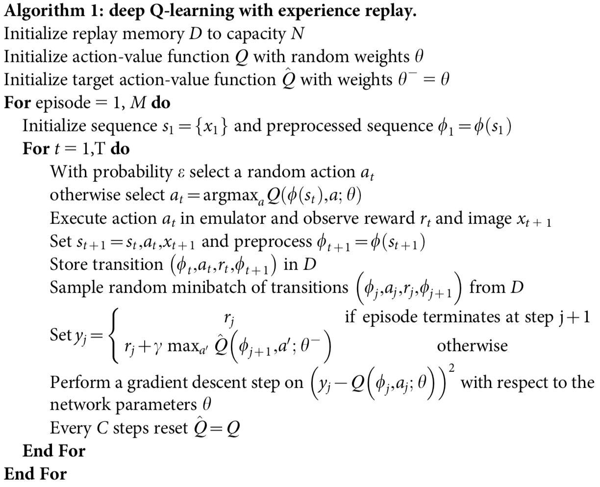
The second modification to online Q-learning aimed at further improving the stability of our method with neural networks is to use a separate network for gen- erating the targets yj in the Q-learning update. More precisely, every C updates we clone the network Q to obtain a target network Q^ and use Q^ for generating the Q-learning targets yj for the following C updates to Q. This modification makes the algorithm more stable compared to standard online Q-learning, where an update that increases Q(st,at) often also increases Q(st 1 1,a) for all a and hence also increases the target yj, possibly leading to oscillations or divergence of the policy. Generating the targets using an older set of parameters adds a delay between the time an update to Q is made and the time the update affects the targets yj, making divergence or oscillations much more unlikely.

简单地说，每隔一段时间copy一次Eval Net成为Target Net减小了每次更新带来的震动，即使得对$Q(s_t,a)$做出的更新不会马上影响到$Q(s_{t+1},a)$

工程实现关键点

1. DQN网络的更新方法：同时初始化两个定义相同的网络，一个是Target Net，一个是Eval Net。前者是作为Q值的目标值出现的一个网络，且其的更新较为落后，往往是Eval Net更新千百轮之后才把后者的参数完全拷贝一份到自身；而后者则是每次学习过程必更新，总是最新的网络参数，用作估计值。
2. 有一个记忆库用来储存之前的记忆，每次训练时随机抽一个batch扔到网络里训练。
3. Fixed Q-targets和记忆库都是打乱经历相关性的机理，也使得神经网络更新更有效率。
4. 刚初始化后的前面n轮是不用网络而完全随机预测的，并把结果存下来训练网络。

核心代码

if (t > learning_starts and
        t % learning_freq == 0 and
        replay_buffer.can_sample(batch_size)):
    # Use the replay buffer to sample a batch of transitions
    # Note: done_mask[i] is 1 if the next state corresponds to the end of an episode,
    # in which case there is no Q-value at the next state; at the end of an
    # episode, only the current state reward contributes to the target
    obs_batch, act_batch, rew_batch, next_obs_batch, done_mask = replay_buffer.sample(batch_size)
    # Convert numpy nd_array to torch variables for calculation
    obs_batch = Variable(torch.from_numpy(obs_batch).type(dtype) / 255.0)
    act_batch = Variable(torch.from_numpy(act_batch).long())
    rew_batch = Variable(torch.from_numpy(rew_batch))
    next_obs_batch = Variable(torch.from_numpy(next_obs_batch).type(dtype) / 255.0)
    not_done_mask = Variable(torch.from_numpy(1 - done_mask)).type(dtype)

    if USE_CUDA:
        act_batch = act_batch.cuda()
        rew_batch = rew_batch.cuda()

    # Compute current Q value, q_func takes only state and output value for every state-action pair
    # We choose Q based on action taken.
    current_Q_values = Q(obs_batch).gather(1, act_batch.unsqueeze(1))
    # Compute next Q value based on which action gives max Q values
    # Detach variable from the current graph since we don't want gradients for next Q to propagated
    next_max_q = target_Q(next_obs_batch).detach().max(1)[0]
    next_Q_values = not_done_mask * next_max_q
    # Compute the target of the current Q values
    target_Q_values = rew_batch + (gamma * next_Q_values)
    # Compute Bellman error
    bellman_error = target_Q_values - current_Q_values
    # clip the bellman error between [-1 , 1]
    clipped_bellman_error = bellman_error.clamp(-1, 1)
    # Note: clipped_bellman_delta * -1 will be right gradient
    d_error = clipped_bellman_error * -1.0
    # Clear previous gradients before backward pass
    optimizer.zero_grad()
    # run backward pass
    current_Q_values.backward(d_error.data.unsqueeze(1))

    # Perfom the update
    optimizer.step()
    num_param_updates += 1

    # Periodically update the target network by Q network to target Q network
    if num_param_updates % target_update_freq == 0:
        target_Q.load_state_dict(Q.state_dict())

Policy Gradient

输入： 状态（State）

输出：直接是动作（Action）（而非Q值）

公式：a=π(s, θ) 或 a=π(a|s, θ)

特点：输出的直接是当前状态下采取各种可能动作的概率。每种动作都可能以其对应概率被选到。另外其相对于基于值的算法如DQN而言可以handle较多action，尤其是连续action空间的问题。

Loss：$$loss=-log(prob(action))*reward$$

核心代码

class Policy(nn.Module):

    def __init__(self):
        super(Policy, self).__init__()

        self.state_space = state_space
        self.action_space = action_space

        self.fc1 = nn.Linear(self.state_space, 128)
        self.fc2 = nn.Linear(128, self.action_space)

    def forward(self, x):
        x = self.fc1(x)
        #x = F.dropout(x, 0.5)
        x = F.relu(x)
        x = F.softmax(self.fc2(x), dim=-1)

        return x

policy = Policy()
optimizer = torch.optim.Adam(policy.parameters(), lr=learning_rate)



def train():

    episode_durations = []
    #Batch_history
    state_pool = []
    action_pool = []
    reward_pool = []
    steps = 0

    for episode in range(num_episode):
        state = env.reset()
        state = torch.from_numpy(state).float()
        state = Variable(state)

        env.render()

        for t in count():
            probs = policy(state)
            c = Categorical(probs)
            action = c.sample()

            action = action.data.numpy().astype('int32')
            next_state, reward, done, info = env.step(action)
            reward = 0 if done else reward # correct the reward
            env.render()

            state_pool.append(state)
            action_pool.append(float(action))
            reward_pool.append(reward)

            state = next_state
            state = torch.from_numpy(state).float()
            state = Variable(state)

            steps += 1

            if done:
                episode_durations.append(t+1)
                plot_durations(episode_durations)
                break

        # update policy
        if episode >0 and episode % batch_size == 0:

            r = 0
            '''
            for i in reversed(range(steps)):
                if reward_pool[i] == 0:
                    running_add = 0
                else:
                    running_add = running_add * gamma +reward_pool[i]
                    reward_pool[i] = running_add
            '''
            for i in reversed(range(steps)):
                if reward_pool[i] == 0:
                    r = 0
                else:
                    r = r * gamma + reward_pool[i]
                    reward_pool[i] = r

            #Normalize reward
            reward_mean = np.mean(reward_pool)
            reward_std = np.std(reward_pool)
            reward_pool = (reward_pool-reward_mean)/reward_std

            #gradiend desent
            optimizer.zero_grad()

            for i in range(steps):
                state = state_pool[i]
                action = Variable(torch.FloatTensor([action_pool[i]]))
                reward = reward_pool[i]

                probs = policy(state)
                c = Categorical(probs)

                loss = -c.log_prob(action) * reward
                loss.backward()

            optimizer.step()

            # clear the batch pool
            state_pool = []
            action_pool = []
            reward_pool = []
            steps = 0

Actor Critic

定义

结合了 Policy Gradient (Actor) 和 Function Approximation (Critic) 的方法. Actor基于概率选行为, Critic 基于 Actor 的行为评判行为的得分, Actor 根据 Critic 的评分修改选行为的概率。简单说，相对于单纯的Policy Gradient，其不再使用回合制更新网络，而是逐步更新网络。而每一步的reward则是由critic网络给出。

优势

可以进行单步更新, 比传统的 Policy Gradient 要快。

劣势

取决于 Critic 的价值判断, 但是 Critic 难收敛, 再加上 Actor 的更新, 就更难收敛. 为了解决收敛问题。

Actor Net

输入：状态（State）
输出：动作（Action）

Critic Net

输入：状态（State）
输出：评价（Reward）

Loss:

$$Loss(policy/actor)=-log\space prob * (reward-critic\space value)\\ Loss(critic)=E[(reward-critic\space value)^2]$$

核心代码

注意虽然看似只写了一个网络，但是因为AC网络的输入相同输出不同，只要最后有两个不同的fc层即可。

import gym, os
import numpy as np
import matplotlib.pyplot as plt
from itertools import count
from collections import namedtuple

import torch
import torch.nn as nn
import torch.optim as optim
import torch.nn.functional as F
from torch.distributions import Categorical

#Parameters
env = gym.make('CartPole-v0')
env = env.unwrapped

env.seed(1)
torch.manual_seed(1)

state_space = env.observation_space.shape[0]
action_space = env.action_space.n


#Hyperparameters
learning_rate = 0.01
gamma = 0.99
episodes = 20000
render = False
eps = np.finfo(np.float32).eps.item()
SavedAction = namedtuple('SavedAction', ['log_prob', 'value'])

class Policy(nn.Module):
    def __init__(self):
        super(Policy, self).__init__()
        self.fc1 = nn.Linear(state_space, 32)

        self.action_head = nn.Linear(32, action_space)
        self.value_head = nn.Linear(32, 1) # Scalar Value

        self.save_actions = []
        self.rewards = []
        os.makedirs('./AC_CartPole-v0', exist_ok=True)

    def forward(self, x):
        x = F.relu(self.fc1(x))
        action_score = self.action_head(x)
        state_value = self.value_head(x)

        return F.softmax(action_score, dim=-1), state_value

model = Policy()
optimizer = optim.Adam(model.parameters(), lr=learning_rate)

def plot(steps):
    ax = plt.subplot(111)
    ax.cla()
    ax.grid()
    ax.set_title('Training')
    ax.set_xlabel('Episode')
    ax.set_ylabel('Run Time')
    ax.plot(steps)
    RunTime = len(steps)

    path = './AC_CartPole-v0/' + 'RunTime' + str(RunTime) + '.jpg'
    if len(steps) % 200 == 0:
        plt.savefig(path)
    plt.pause(0.0000001)

def select_action(state):
    state = torch.from_numpy(state).float()
    probs, state_value = model(state)
    m = Categorical(probs)
    action = m.sample()
    model.save_actions.append(SavedAction(m.log_prob(action), state_value))

    return action.item()


def finish_episode():
    R = 0
    save_actions = model.save_actions
    policy_loss = []
    value_loss = []
    rewards = []

    for r in model.rewards[::-1]:
        R = r + gamma * R
        rewards.insert(0, R)

    rewards = torch.tensor(rewards)
    rewards = (rewards - rewards.mean()) / (rewards.std() + eps)

    for (log_prob , value), r in zip(save_actions, rewards):
        reward = r - value.item()
        policy_loss.append(-log_prob * reward)
        value_loss.append(F.smooth_l1_loss(value, torch.tensor([r])))

    optimizer.zero_grad()
    loss = torch.stack(policy_loss).sum() + torch.stack(value_loss).sum()
    loss.backward()
    optimizer.step()

    del model.rewards[:]
    del model.save_actions[:]

def main():
    running_reward = 10
    live_time = []
    for i_episode in count(episodes):
        state = env.reset()
        for t in count():
            action = select_action(state)
            state, reward, done, info = env.step(action)
            if render: env.render()
            model.rewards.append(reward)

            if done or t >= 1000:
                break
        running_reward = running_reward * 0.99 + t * 0.01
        live_time.append(t)
        plot(live_time)
        if i_episode % 100 == 0:
            modelPath = './AC_CartPole_Model/ModelTraing'+str(i_episode)+'Times.pkl'
            torch.save(model, modelPath)
        finish_episode()

if __name__ == '__main__':
    main()

DDPG

定义

输入： 状态（State）

输出：直接是动作（Action）（而非Q值）

公式：a=π(s, θ) 或 a=π(a|s, θ)

特点：输出的直接是当前状态下采取各种可能动作的概率。每种动作都可能以其对应概率被选到。

应用场景：连续行为场景

由来

在RL领域，DDPG主要从：PG -> DPG -> DDPG 发展而来。
Deepmind在2016年提出DDPG，全称是：Deep Deterministic Policy Gradient,是将深度学习神经网络融合进DPG的策略学习方法。
相对于DPG的核心改进是： 采用卷积神经网络作为策略函数μ和Q函数的模拟，即策略网络和Q网络；然后使用深度学习的方法来训练上述神经网络。
Q函数的实现和训练方法，采用了Deepmind 2015年发表的DQN方法。

原理图

算法